Our discussion thus far has mostly been built on text, so in this section we will present and explain the graphical outcomes. If you are interested in a hands-on example of how the early PEAR experiments looked from an operator's point of view, you can view our demonstration animation, watch the PEAR Proposition DVD, or even purchase an REG-1 to run the experiment in your own home.

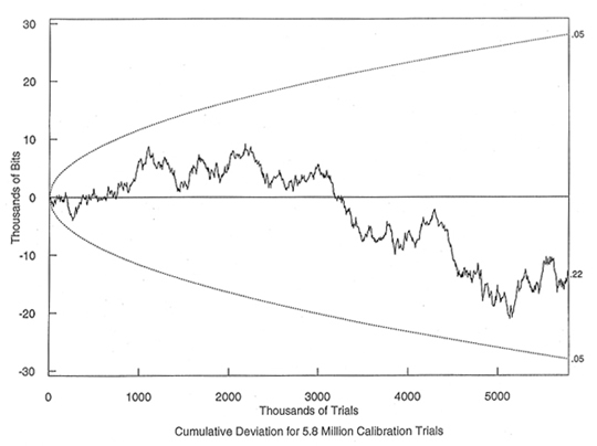
The first graph below this paragraph shows the output behavior of the REG when run in calibration mode. To understand the graph, think back to our heads and tails analogy. The X-axis of the graph (the part that moves from left to right) roughly represents the number of coin flips that were accumulated. As you move further along the graph to the right, it means that more time has passed by and that you have more coin flips. The Y-Axis (the one in the up and down direction) represents the deviation from chance. If this sounds confusing, remember our analogy.

If a coin were flipped 10 times, we would expect to see about 5 heads. The "deviation from chance" in this case would be the number of heads that we actually counted, minus the expected value of five. So, 7 heads on 10 coin flips would represent a deviation of +2, which means we would move upward from zero on the graph. Three heads would represent a deviation of -2, which means we would move down from the zero line by two. So, in looking at this graph, you might notice that at 3,000 (thousand) trials, or 3 million trials, there is a deviation of about +5,000 bits. At the PEAR lab, one trial constituted 200 coin flips, so we find that out of 600 million coin flips (which we'll refer to as bits from now on), about 300,005,000 came out as heads (which we'll now refer to as "1 bits") and about 299,995,000 came out as tails (which we'll now call "0 bits".)

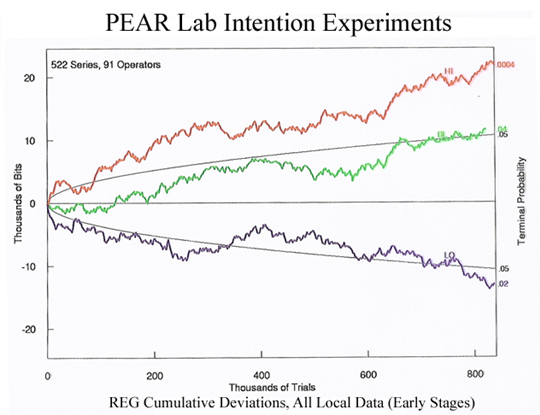
The next graph shows the output of the REG when operators were attempting to have an influence. The red line shows the output when operators were trying to go "high" (create more 1 bits), the green when operators tried to keep the results to the center, and the blue line shows when operators tried to go "low" (create more 0 bits.) As you can probably see, there is a bit of a difference between the operators' active intention data, and the data that resulted when the box was running by itself in calibration mode.

The final point that we should make about these data involves some technical details about the experiment and statistical significance. When you heard about the calibration data, you may have thought back to our earlier example and said "Well, is it significant to find 300,005,000 heads if I flip a coin 600 million times?" The answer is no, but perhaps first we should define significance. In the case of a statistical experiment, experimenters usually use some kind of standard criteria to determine whether or not a result is "significant" from a statistical point of view.

In most cases, an experimental result is considered significant if the probability of obtaining it by chance less than 1 in 20 (or sometimes 1 in 100, depending on the field.) This means that if you ran a full experiment 20 times and there was no effect at all, you would only expect to find that one of your experiments randomly created results at the 1 in 20 level. Essentially, a result is considered statistically significant if there is only a small probability that you would see the observed results if there really was no effect.

Since it would be tedious to calculate statistical significance for every single set of outcomes, PEAR was kind enough to include parabolas on its graph to accomplish this purpose. Put as simply as possible, any line that ends "inside" the parabola is considered to be statistically insignificant - it represents a result that we would generally expect to find by chance. On the other hand, results that end outside of the parabola are less likely to occur by chance to the extent that they are outside of it. If you look at the intention data, the "P=.02" next to the low data means that there is only about a 2 in 100 chance of an experiment with no effect producing a deviation that is at least that strong in the low direction. The P=.0004 in the high direction means that the odds of that result occurring by chance are only about 4 in 10,000.

If you combine these results together, the probability of such a result occurring by chance is less than 1 in 100,000; whereas the calibration data behaved exactly as we would expect a perfect coin to behave. More interestingly, this data only represents the first few years of PEAR experiments, and it includes EVERY operator. In the decades that followed, the trend continued, which means that its statistical significance grew exponentially. As of the last count, the probability of the lab obtaining results like these due to chance are less than 1 in 1,000,000,000,000. In short, it is almost impossible that these effects occurred due to chance.